My very first quarto document

Autore/Autrice

Jane Doe

Data di Pubblicazione

23 luglio 2025

Ta-dan

ggplot2 is an R (R Core Team 2025) package developed by (Wickham 2016). Epifania, Anselmi, e Robusto (2024) published an interesting paper on Linear Mixed Effects Models.

R Core Team. 2025. R: A Language and Environment for Statistical Computing. Vienna, Austria: R Foundation for Statistical Computing. https://www.R-project.org/.

Wickham, Hadley. 2016. ggplot2: Elegant Graphics for Data Analysis. Springer-Verlag New York. https://ggplot2.tidyverse.org.

Epifania, Ottavia M, Pasquale Anselmi, e Egidio Robusto. 2024. «A guided tutorial on linear mixed-effects models for the analysis of accuracies and response times in experiments with fully crossed design.» Psychological Methods. https://doi.org/https://doi.org/10.1037/met0000708.

Quarto

Show this code

ggplot(mtcars, aes(hp, mpg, color = factor(am))) +
  geom_point() +
  geom_smooth(formula = y ~ x, method = "loess") +
  theme(legend.position = 'bottom')

Codice

```{r}
#| column: margin

lm(hp ~ mpg*am, data = mtcars)
```


Call:
lm(formula = hp ~ mpg * am, data = mtcars)

Coefficients:
(Intercept)          mpg           am       mpg:am  
   360.7425     -11.6916      32.3404       0.7768

Codice

datatable(mtcars,
  options = list(pageLength = 5))

Quarto enables you to weave together content and executable code into a finished document. To learn more about Quarto see https://quarto.org.

I want this picture displayed in the margin

First column, 4/12 of the toal width

Second column, 8/12 of the total width

Running Code

When you click the Render button a document will be generated that includes both content and the output of embedded code. You can embed code like this:

Codice

lm(hp ~ mpg*am, data = mtcars)


Call:
lm(formula = hp ~ mpg * am, data = mtcars)

Coefficients:
(Intercept)          mpg           am       mpg:am  
   360.7425     -11.6916      32.3404       0.7768

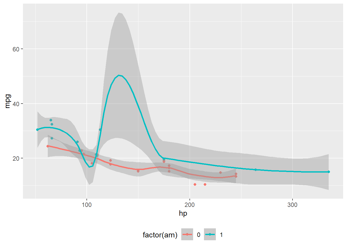
Tabella 1 presents two datasets: Tabella 1 (a) is cars and Tabella 1 (b) is pressure

Codice

library(knitr)
kable(head(cars))
kable(head(pressure))

Tabella 1: Datasets

(a) Cars

speed	dist
4	2
4	10
7	4
7	22
8	16
9	10

(b) Pressure

temperature	pressure
0	0.0002
20	0.0012
40	0.0060
60	0.0300
80	0.0900
100	0.2700

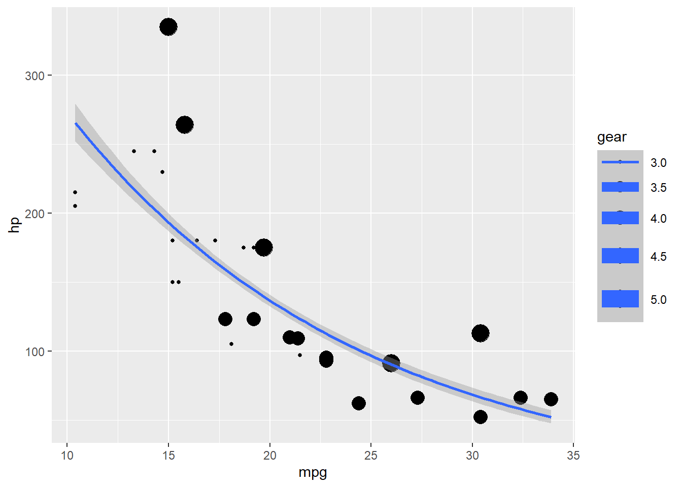
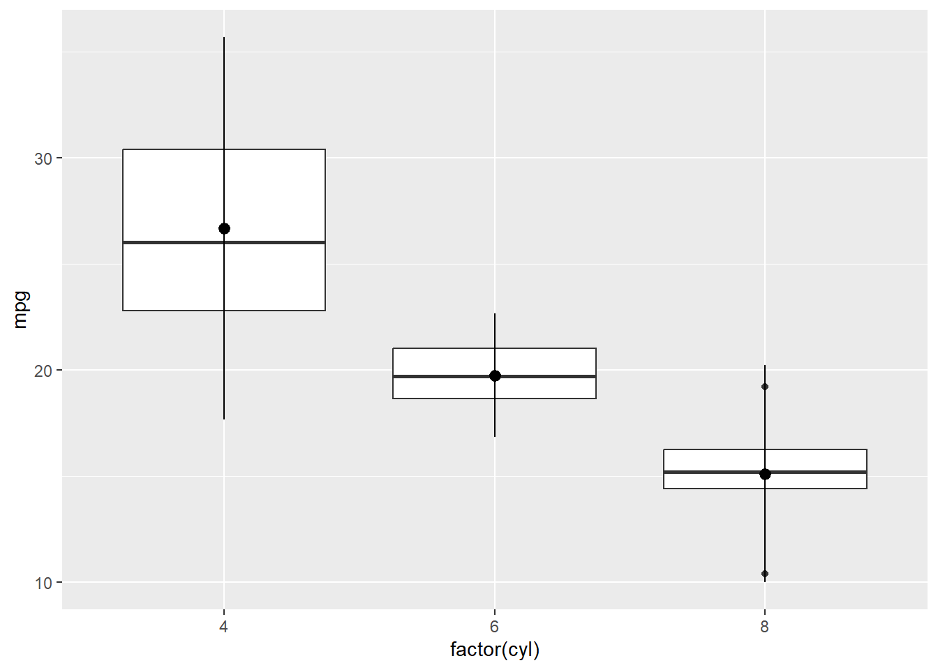
Figura 1 illustrates different things. Figura 1 (a) illustrates this, Figura 1 (b) illustrates that and so on

You can add options to executable code like this

[1] 4

The echo: false option disables the printing of code (only output is displayed).

--- title: "My very first quarto document" author: "Jane Doe" date: today format: html: theme: light: journal dark: superhero toc: true toc-location: left code-fold: true code-tools: true grid: sidebar-width: 300px body-width: 900px margin-width: 300px gutter-width: 1.5rem lang: it execute: echo: true message: true error: true bibliography: references.bib citation-location: margin --- ```{r} #| include: false library(ggplot2) library(DT) ``` # Ta-dan `ggplot2` is an R [@rsoft] package developed by [@ggplot]. @epifania2024 published an interesting paper on Linear Mixed Effects Models. ## Quarto ```{r} #| echo: fenced #| column: margin lm(hp ~ mpg*am, data = mtcars) # <1> ``` ```{r} #| code-fold: true #| code-summary: "Show this code" ggplot(mtcars, aes(hp, mpg, color = factor(am))) + geom_point() + geom_smooth(formula = y ~ x, method = "loess") + theme(legend.position = 'bottom') ``` ```{r} #| column: margin datatable(mtcars, options = list(pageLength = 5)) ``` Quarto enables you to weave together content and executable code into a finished document. To learn more about Quarto see <https://quarto.org>. ::: {.column-margin} I want this picture displayed in the margin ![](slides/01-Baby-steps/img/peacock.png) ::: ::: {.grid} ::: {.g-col-4} First column, 4/12 of the toal width ::: ::: {.g-col-8} Second column, 8/12 of the total width ::: ::: ## Running Code When you click the **Render** button a document will be generated that includes both content and the output of embedded code. You can embed code like this: ```{r} #| column: margin lm(hp ~ mpg*am, data = mtcars) ``` ```{r} #| fig-column: margin #| echo: false ggplot(mtcars, aes(hp, mpg, color = factor(am))) + geom_point() + geom_smooth(formula = y ~ x, method = "loess") + theme(legend.position = 'bottom') datatable(mtcars, options = list(pageLength = 5)) ``` @tbl-tables presents two datasets: @tbl-tables-1 is cars and @tbl-tables-2 is pressure ```{r} #| label: tbl-tables #| tbl-cap: "Datasets" #| tbl-subcap: #| - "Cars" #| - "Pressure" #| layout-ncol: 2 library(knitr) kable(head(cars)) kable(head(pressure)) ``` @fig-plotsModels illustrates different things. @fig-plotsModels-1 illustrates this, @fig-plotsModels-2 illustrates that and so on ```{r} #| label: fig-plotsModels #| echo: false #| warning: false #| column: screen-inset-shaded #| layout-nrow: 2 #| layout-ncol: 2 #| fig-cap: "One dataset, different models" #| fig-subcap: #| - "The data" #| - "Polynomial" #| - "Linear Model" #| - "GLM with Poisson" ggplot(mtcars, aes(mpg, hp, size = gear)) + geom_point() ggplot(mtcars, aes(mpg, hp, size = gear)) + geom_point() + geom_smooth() ggplot(mtcars, aes(mpg, hp, size = gear)) + geom_point() + geom_smooth(method = "lm") ggplot(mtcars, aes(mpg, hp, size = gear)) + geom_point() + geom_smooth(method = "glm", method.args = list(family = "poisson")) ggplot(mtcars, aes(x = factor(cyl), y = mpg)) + geom_boxplot() + stat_summary(fun.data=mean_sdl, geom="pointrange", color="black") ``` You can add options to executable code like this ```{r code} #| echo: false 2 * 2 ``` The `echo: false` option disables the printing of code (only output is displayed).